Your LLM Is Carrying Around an Entire Library Every Time It Answers You
How KIVI, TokenSelect, SnapKV, TopK-Flash, and MLA each try to solve the KV-cache bottleneck — with real experiments on Llama-2-7B running on H100 GPUs

Every time you ask ChatGPT a question, something slightly absurd happens behind the scenes.
The model rereads its entire conversation history over and over again.
Not metaphorically. Literally.
Imagine writing a new sentence in an essay, but before writing every single word, you first reread every page you’ve already written. That is essentially what autoregressive decoding does.
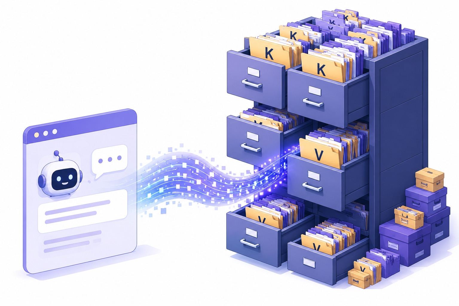
Modern LLMs avoid recomputing everything from scratch by storing intermediate attention information in something called the KV cache. The cache is one of the main reasons LLMs are fast enough to be usable at all.
It is also one of the biggest reasons inference becomes painfully expensive at long context lengths.
As prompts grow from 4K → 32K → 128K tokens, the KV cache starts behaving less like a helpful optimization and more like a storage unit the GPU has to drag around everywhere.
In this project, we implemented and benchmarked five different approaches for dealing with this problem:
KIVI → compress the cache with quantization
TopK / TokenSelect → only attend to important tokens
TopK-Flash → make sparse attention work at very long context
SnapKV → decide once which tokens matter, then throw the rest away
MLA → redesign the cache representation entirely
All experiments were run on Llama-2-7B-chat-hf using NVIDIA H100 80GB GPUs.
And the results were surprisingly different from what we initially expected.
Part 1: What Even Is the KV Cache?
To understand the KV cache, you first need to understand what attention is actually doing.
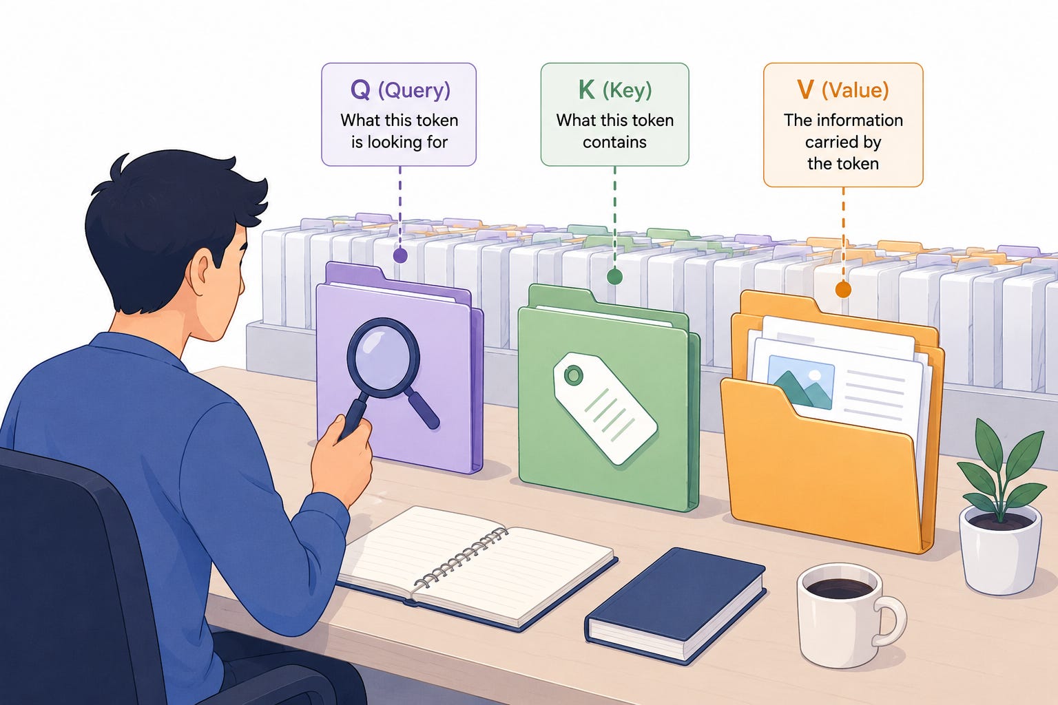
When a transformer processes text, every token creates three vectors:
Query (Q) → what this token is looking for
Key (K) → what this token contains
Value (V) → the actual information carried by the token
Attention works by comparing Queries against Keys:
Then using those scores to mix together the Values:
You can think of it like searching through notes.
Queries are the search terms.
Keys are the labels on the folders.
Values are the contents inside the folders.
When generating text token-by-token, the model has to repeatedly search through all previous tokens.
Without caching, this becomes extremely wasteful.
If the prompt has 4,000 tokens, then every newly generated token would require recomputing Keys and Values for all 4,000 earlier tokens again.
That would be like reopening and relabeling every folder in the library every time someone asks for one document.
So instead, the model stores all previously computed Keys and Values in GPU memory.
That storage is the KV cache.
The Problem: The Cache Never Stops Growing
The KV cache sounds great until you realize how large it becomes.
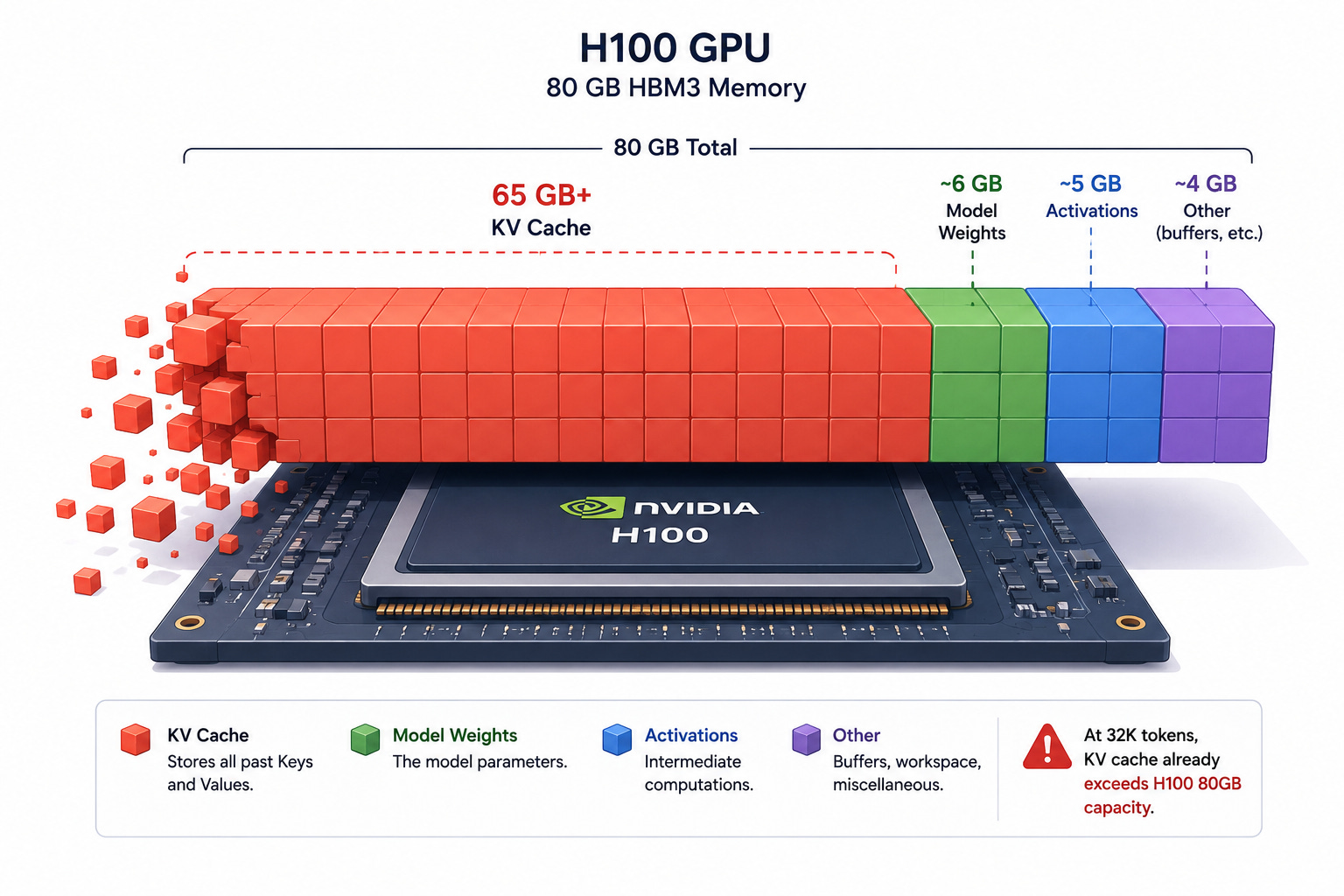
For Llama-2-7B:
where L = layers, H = heads, D = head dimension, S = sequence length, B = batch size, b = bytes per element. The leading 2 accounts for both K and V.
At 32 layers, 32 attention heads, sequence length = 4096, batch size = 32, and FP16 precision, the KV cache alone requires 65.5 GB.
That is just the cache. Not the model weights. Not activations. Not optimizer state. Just the memory needed to remember previous tokens.
An H100 has 80 GB total.
So the GPU starts spending most of its life carrying around memory instead of doing actual computation.
This is why modern LLM inference is often memory-bandwidth bound rather than compute-bound.
Decode-step attention has very low arithmetic intensity: you reread the entire KV cache to compute a tiny amount of work per token. That is what memory-bandwidth bound actually means.
The GPU cores are fast enough. The problem is moving massive KV tensors back and forth from HBM every decode step.
It is similar to having an extremely fast chef in a kitchen where ingredients are stored half a mile away. The chef spends more time waiting for ingredients than cooking.

That is the KV-cache bottleneck.
Part 2: Five Different Ways to Solve the Problem
The interesting thing about KV-cache optimization is that different methods attack completely different parts of the problem.
Some try to make the cache smaller. Some try to read less of it. Some try to reorganize it. And some try to redesign the entire representation.
Strategy 1 - KIVI: Shrink the Cache with Quantization
Core Idea
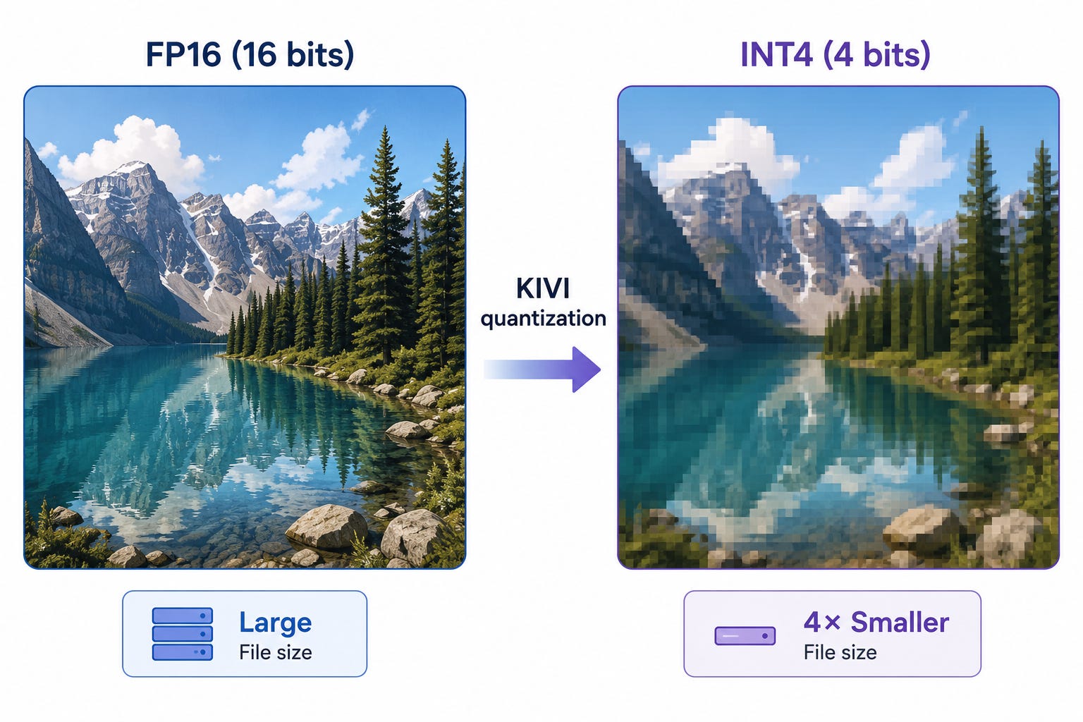
Instead of storing Keys and Values in 16-bit floating point format, store them in 2-bit or 4-bit integers.
Same cache. Much fewer bits.
It is similar to compressing a RAW image into a JPEG. The image is slightly less precise, but dramatically smaller.
How KIVI Works
KIVI makes an important observation: Keys and Values behave differently statistically.
Keys vary more across dimensions than across tokens. So KIVI quantizes them per-channel — each dimension gets its own scale factor.
Values vary more across tokens. So KIVI quantizes them per-token.
This asymmetric design preserves much more quality than naive quantization.
So 4-bit storage gives 4× compression, and 2-bit gives 8×, since the baseline is 16-bit FP16.
KIVI also keeps the newest 128 tokens in full FP16 precision. Why? Because recent tokens are the ones the model attends to most heavily. Older tokens matter less precisely.
You can think of this like photo compression on your phone: recent photos stay high resolution, while older archived photos get compressed aggressively.
The implementation used Triton kernels for INT4 packing, CUDA kernels for on-the-fly dequantized attention, and custom packed KV formats.
The Results
At low batch size, KIVI was actually slower than baseline. That surprised us.
Throughput results (tokens/sec):
Batch Size   Baseline (tok/s)   KIVI 4-bit (tok/s)
----------   ----------------   ------------------
  1           70                30
  4           242               123
  16          438               480
  32          497               957
  64          OOM               1295
  128         OOM               1517
The crossover happens at BS=16 (KIVI overtakes baseline 480 vs 438 tok/s)
and reaches 1.93× at BS=32 (957 vs 497). KIVI also extends the maximum
batch size from 32 to 128, raising single-GPU peak throughput by ~3×.
Why? Because at low batch size, the overhead of dequantization outweighs the bandwidth savings. But once batch size grows, memory movement dominates runtime, and KIVI wins massively.
At BS=32, baseline reached 497 tok/s while KIVI 4-bit hit 873 tok/s — while using dramatically less memory.
Even more impressive: KIVI 4-bit was essentially lossless on LongBench. The overall score was 0.291 for baseline versus 0.292 for KIVI 4-bit.
So the model barely cared that historical KV tensors were compressed.
Strategy 2 - TopK / TokenSelect: Only Read Important Tokens
Core Idea
Maybe the model does not actually need to attend to every token during every decode step.
Instead of compressing the cache, keep the cache full precision but only attend to the most relevant parts.
This is similar to studying for an exam. You probably do not reread the entire textbook every five minutes. You skim the important pages.
That is exactly what TopK does.
How TopK Works
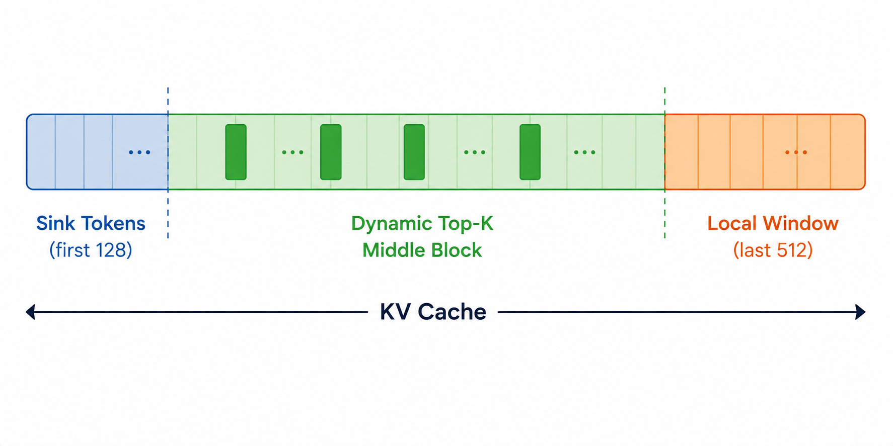
The KV cache is divided into three regions:
1. Sink Tokens. The first 128 tokens are always kept. These are called attention sinks. Transformers have a strange behavior where early tokens attract attention even when semantically unimportant. Removing them caused catastrophic quality collapse. The model behaves like those first tokens are structural anchors.
2. Local Window. The most recent 512 tokens are always kept. This makes intuitive sense — recent context is usually the most relevant.
3. Dynamic Top-K Tokens. For the middle portion of the sequence, the model dynamically scores tokens and selects the most relevant K positions.
A custom Triton kernel fused Q·Kᵀ, softmax, cross-head reduction, and top-K selection into a single launch. The method also reused selections when consecutive queries were highly similar.
The Results
At K=1024, TopK matched baseline quality almost exactly.
But one result stood out: TopK actually outperformed baseline on TriviaQA.
Why? Because TriviaQA answers are often concentrated in small sections of text. TopK acts almost like retrieval — it filters away irrelevant filler and forces attention toward answer-heavy regions.
The downside: at short context lengths, the scoring overhead itself becomes expensive. At batch size 1, baseline reached 70 tok/s while TopK only managed 43 tok/s. At 1K–4K context, the model spends too much time deciding what to attend to. But at very long context lengths, sparse attention becomes increasingly worthwhile.
Strategy 3 - TopK-Flash: Sparse Attention at 32K+
TopK works well conceptually. But scaling it to 32K–64K context introduces another problem: allocating gigantic contiguous KV tensors becomes painful.
So instead of storing KV as one massive block, TopK-Flash organizes memory into pages.
The Paged KV Idea
Think of this like virtual memory in operating systems. Instead of storing one giant continuous book, the cache is split into many smaller pages. Each page stores 256 tokens.
The model can then selectively attend to pages without moving memory around. Flash Attention handles the sparse page lookup directly, avoiding expensive gathering operations.
The Results
At 32K context, TopK-Flash dropped time-to-first-token from 2627 ms to 1761 ms — a 33% reduction. Peak memory dropped from 52.1 GB to 42.1 GB
Metric           Baseline    TopK-Flash
--------------   --------    ----------
TTFT (32K)       2597 ms     1761 ms
Peak Memory      52.1 GB     42.1 GB
64K Context      OOM         supported.
And unlike baseline, it could handle 64K context without OOM.
Interestingly, decode throughput stayed roughly similar. The main improvement came from memory allocation behavior and reduced prefill overhead.
Strategy 4 - SnapKV: Decide Once and Commit
Most sparse-attention methods rescore tokens during every decode step. SnapKV asks: what if we made the selection once during prefill and never changed it?
How SnapKV Works
After processing the prompt, SnapKV looks at the attention patterns of the last few prompt tokens. Those tokens effectively reveal what the model currently considers important.
The method collects attention from the last 32 query positions, assigns vote scores to earlier tokens, smooths the scores with max pooling, keeps only the top 40% of tokens, and permanently evicts everything else.
After that, decode proceeds normally. No per-step scoring. No dynamic selection overhead.
It is similar to studying for an exam. As you skim the last few pages of your notes, you naturally start highlighting which earlier sections matter most. SnapKV does exactly that: it watches what the prompt's final tokens pay attention to and uses those signals to decide which earlier tokens are worth keeping. Once the highlighting is done, you do not reread the textbook during the exam, you trust the highlights.

The Results
SnapKV was probably the most surprising method. It compressed the cache and slightly improved quality.
Overall LongBench quality went from 0.291 (baseline) to 0.295 (SnapKV). On TriviaQA, scores jumped from 0.644 to 0.687.
Why did quality improve? Because the observation-window voting acted like a lightweight retrieval system. It removed irrelevant tokens before generation even started.
The method struggled more on tasks like Qasper, where evidence is scattered throughout long documents. If the relevant information is distributed broadly, one-shot eviction can throw away useful context. But for concentrated-context tasks, SnapKV was remarkably robust.
Strategy 5 - MLA: Change the Representation Entirely
All previous methods still store some form of Keys and Values. MLA takes a completely different approach. Instead of storing full KV tensors, it stores a compressed latent representation.
The Core Idea
Rather than saving K and V tensors, MLA stores a compressed latent vector c, and reconstructs approximate Keys and Values during attention.
This is similar to storing a ZIP file instead of the original folder. You do not keep every file expanded all the time — you reconstruct them when needed.
The Results
KV cache size dropped 3.9× — from 1207 MB to 311 MB at 2048-token prefill.
Decode throughput rose from ~34 tok/s (MLA baseline) to 43 tok/s (MLA), a 1.26–1.32× speedup at batch size 1 across prefill lengths 512–2048.
The decode speedup was real, even at batch size 1. That was important because it confirmed that decode was fundamentally bandwidth-bound. Less KV memory directly translated into faster inference.
But the quality collapse was severe. LongBench dropped from 0.291 (baseline) to 0.081 (MLA).
The checkpoint we used had rank-8 latent compression and only 2048-token training context, which was too aggressive for 4K retrieval-heavy tasks. So MLA demonstrated the potential of latent KV representations, but not yet production-ready quality for this setup.
Part 3: Comparing the Methods
The most interesting takeaway from this project was that there was no universally best method. Each method optimized a different bottleneck.
KIVI 4-bit — best for high-throughput batch serving
TopK — best for sparse long-context attention
TopK-Flash — best for 32K–64K context serving
SnapKV — best for quality-neutral practical compression
MLA — best as an architectural long-term redesign
KIVI was the strongest overall deployment result. SnapKV was the most surprisingly elegant. TopK-Flash solved real long-context memory issues. And MLA hinted at where future architectures may go.
All raw throughput sweeps, memory traces, and per-task quality scores from the five strategies above are logged on the public Weights & Biases dashboard: 📊 https://wandb.ai/rm4318-columbia-university/kv-cache-hpml
Part 4: What Surprised Us Most
1. Quantization Does Not Automatically Improve Latency
We initially assumed smaller KV tensors would always be faster. Not true. At low batch size, the GPU was not bandwidth-bound enough for quantization savings to matter. The dequantization overhead dominated instead.
2. Attention Sink Tokens Are Extremely Important
Removing sink tokens immediately destroyed quality. Those first few tokens behave almost like structural reference points for the transformer — even when semantically meaningless.
3. SnapKV Was Much More Stable Than Expected
At first glance, permanently deleting 60% of the prompt before generation sounds dangerous. But the model’s own late-prefill attention patterns turned out to be surprisingly predictive of future relevance.
4. MLA’s Problem Was Training, Not the Idea Itself
The compression worked. The memory savings worked. The speedup worked. The issue was that the checkpoint had not been trained broadly enough for long-context retrieval. That makes MLA feel more like a future architectural direction than a failed method.
Part 5: Can We Combine These Methods?
The five strategies above each attack a different part of the problem. KIVI shrinks each token. TopK reads fewer tokens. SnapKV decides once which tokens matter. MLA changes the representation entirely.
A natural question is whether these methods compose. If their assumptions are orthogonal, and they mostly are, then stacking them should stack the savings.
We tested the cleanest version of this idea: combine KIVI’s INT4 storage with TopK’s sparse selection. Store the cache compressed and only attend to a subset of it.
What worked
At 32K context, peak memory dropped from 52.1 GB to 25.8 GB. A 50% reduction, larger than either method individually. LongBench quality stayed at 0.297, essentially identical to baseline 0.291. The compression was semantically lossless.
So the memory story was exactly what we hoped for. Two orthogonal compression axes, two stacked savings.
What didn’t
Decode throughput regressed by 39%. Baseline ran at 21.0 tok/s; the hybrid ran at 12.9 tok/s.
Two things went wrong, both fixable in principle:
The scoring kernel still has to read the full INT4 K cache to figure out which tokens to attend to. So even though the actual attention computation only touches a small subset, the scoring pass touches everything. That cancels much of the bandwidth benefit of sparse selection.
And at batch size 1, INT4 GEMV inherits the same dequantization overhead that hurt standalone KIVI at low batch, except this time there’s no large batch to amortize it against.
Neither of these is fundamental. A fused kernel that combines scoring, selection, and INT4 attention into a single pass, analogous to what FlashAttention does for dense attention, should recover most of the latency. A hierarchical scoring scheme that scores at the page level first and only drills down for shortlisted pages would reduce the O(S) scoring cost toward O(K).
The orthogonal memory savings are real and additive. The throughput gap is an engineering problem, not an algorithmic one.
What’s next: SnapKV × KIVI
The KIVI×TopK experience suggests a better composition for follow-up work: SnapKV followed by KIVI.
SnapKV’s appeal in this setting is that it does its work once, at the end of prefill, and leaves nothing to be done during decode. There’s no per-step scoring kernel, no token-by-token gather, no scoring pass that cancels out the bandwidth savings. Once SnapKV finishes, the cache is just smaller, and a smaller cache is exactly what KIVI’s INT4 storage wants as input.
The arithmetic is appealing. SnapKV at r=0.4 reduces the cache to roughly 2.5× smaller. KIVI 4-bit compresses what remains by another 4×. Stacked, that’s a 10× reduction in KV memory with the per-step decode path identical to standalone KIVI, the very regime where KIVI is fastest. No fused-kernel engineering required to capture the win.
The interesting open question is whether the two methods interact gracefully. SnapKV evicts based on attention vote scores; KIVI’s quantization noise will shift those scores slightly. If the eviction is done first (on FP16 attention patterns) and quantization second, the interaction should be clean. We expect the combination to inherit SnapKV’s quality preservation and KIVI’s throughput crossover at BS≥16. That’s the experiment we want to run next.
Conclusion
The KV cache is becoming one of the defining systems bottlenecks of modern LLM inference. As context windows grow larger, models spend increasing amounts of time moving memory rather than performing computation.
The five approaches we explored each make a different assumption about the structure of attention:
KIVI assumes KV tensors are numerically compressible.
TopK assumes attention is sparse.
TopK-Flash assumes sparse attention matters even more at long context.
SnapKV assumes future relevance is predictable from the prompt.
MLA assumes the KV representation itself is low-rank.
What makes this area exciting is that these assumptions are not mutually exclusive. A future system could combine quantized KV storage, sparse page-based attention, and latent representations all in one inference stack.
In many ways, KV-cache optimization is starting to resemble classical computer systems engineering. We are suddenly thinking again about caching, paging, compression, memory hierarchy, bandwidth, locality, and allocation patterns.
Except now the “program” is a 7B-parameter language model trying to remember a 64K-token conversation. And that turns out to be a fascinating systems problem.
So the next time ChatGPT pauses for a beat before answering, it is not thinking. It is moving memory.
This project was completed as part of HPML Spring 2026 at Columbia University, advised by Dr. Kaoutar El Maghraoui. All experiments ran on NVIDIA H100 80 GB GPUs via Modal cloud infrastructure. Full code, benchmark scripts, and result files, are in the GitHub repository: 🔗 https://github.com/rishika1099/KV-Cache-Implementation
 | A guest post by
|
This is one of the clearest breakdowns of KV cache optimization I've read. The "chef waiting for ingredients half a mile away" analogy for memory-bandwidth-bound inference is going to stick with me. Really well-structured comparison across five very different approaches!